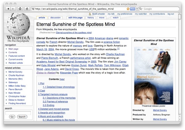
It’s pretty clear to computer science geeks that Directed Edge is supposed to be doing groovy things with graphs. In fact our recommendation engine, and some of the things that are unique about our approach to recommendations, are built on our super-fast graph database. When we went live yesterday with the latest version of our recommendations web services, another, much bigger thing happened behind the scenes for us: we cut over to the new version of our graph database.
Every time that Directed Edge gets mentioned in nerdier circles we get a lot of questions about this fabled graph-engine, so we thought we’d indulge our techie friends with some background info.
When we first decided to build the Directed Edge engine, we’d built some in-memory and RDF-store based prototypes to start hashing out the recommendations algorithms, but the RDF stores couldn’t keep up performance-wise and staying memory-based obviously wasn’t an option for persistent data. So we tried porting things over to SQL-based databases … and got a working version, but it was so painfully slow that we knew we needed to keep looking. The initial version of our web services were built on simply serializing data objects to disk and reading records from index files that we loaded up into memory. This worked and was both fast and memory efficient, but ignored most of the harder problems of a true database.
What are those performance characteristics, exactly? Well, it’s fuzzy where the cut-off is, but we’re now able to import a graph with 2.5 million nodes and 60 million edges in 12 minutes on a MacBook. Query times for finding related items on a similarly large graph with warm disk-buffers average under 5 ms.
With the latest version of our web services and database, we’ve gone from having a graph-store to having a proper graph database. We now use straight memory-mapped I/O, disk-based linear-hashing, have mechanisms to address data fragmentation, thread-safe read / write locking and logging / log replaying.
Before we jump into the computer-science-y core of what we’re doing, I’ll throw down some nerd-cred, and give some perspective to the design decisions made. The design was done by me, Directed Edge’s CTO, and I’ve been looking at algorithms for graph-based similarity for around 5 years now. During the earlier half of the decade I did a series of talks on “contextual webs” to our crew in the Linux world. While I have no academic background in database design, I’ve been doing low level bit-wrangling for most of the last decade and Directed Edge’s data backend is the third key-value store that I’ve written from the ground up. So, what I’m trying to say is: some of these ideas may be original, many are not, some fly in the face of traditional database design which is likely some mix of novel and naive. Be that as it may, the closest that we’ve gotten to our performance using off the shelf databases was with BDB with 5% of the throughput of our database.
So, on to geekery. Let’s start at the top level of abstraction and work our way down. The impatient may feel free to turn the page at any time since the juicer bits are in the lower levels. Â We’ve tried to bold the highlights.
The Store: Items, Links, References, Tags and Whathaveyou.
Sitting up on top of the architecture is a C++ class called “Store”. Like the rest of the things that sit below the web services (which are in Java), it’s written in C++. This is the API that we use to deal with a database. To our recommendations code, this is the database.
Things are pretty simple there, and the API is flexible enough that it’s let us swap out the implementation below it to compare other backends. Basically it’s this:
- The store is a big collection of items, which can be anything — a user, a product, a web page.
- Items are identified by a string unique identifier which maps to an integer index.
- We can look up an item’s index by name really quickly.
- Items have links and references, which are basically a list of things they’re connected to and things that connect to them. These are symmetrical — so creating a link from item A to item B, creates a reference from item B to item A.
- Items can also have tags, e.g. “user”, “product”, “musician”, “film” and so on. Tags are non-exclusive, so an item can have as many tags as appropriate.
- Links and references can have weights of 1 to 10 or be unweighted. We use that for ratings. So a rating is just a link from user A to product B with weight of 1 to 10.
- We can also store arbitrary other fields along with these like “text”. Really, the only limitations on what can be associated with an item are what we choose to expose in the API here. The lower levels are flexible.
So that’s the top level. That’s what makes things look like a nice, clean graph architecture without mucking with all of the lower-level storage details. At this level everything’s thread-safe too, so the map-reduce pattern that we use when generating recommendations doesn’t leave a trail of destruction and SIGBADTHINGSs in its wake.
Things Start Looking Databasey: Rows and Columns
Like traditional databases, our database is organized into rows and columns. An item is just a row. Unlike most databases, there’s only one set of rows (only a small lie, which we’ll ignore for convenience), and the primary things contained in rows are lists.
There are really no huge surprises here:
- A database has a list of columns, a stack of deleted rows (to recycle indexes) and a row count.
- Adding a row to the database adds a row to all columns.
- There’s a flag for if a column is hashed or not, which enables fast lookups and requires unique data values.
- There’s a basic column type that just stores byte arrays and a bunch built on top of it for storing things like link and reference vectors, string lists, strings and so on.
- Any field in an item can be empty and all of our column data types have sane values for empty contents, which are returned if the data pointer for a row is set to null.
Column Locking
We’ve got two types of locks that we use, one surprisingly boring, one a little more creative.
The most important fields in the Directed Edge database are the links and references. They convey things like “which pages are linked on this website” or “which products has this customer bought” or “which news items has this user clicked on”. Those lists are of the type IndexVector within our database and have their own special kind of lock.
The rest of the columns use normal read-write locks. We use an array of 8 read-write locks per column. When lock request comes in it is hashed by shifting the index by three bits and then issues a lock on the column. We found this in practice to be faster than keeping a table or tree of locks since maintaining that tree would require a single read-write lock for the tree maintenance and contention for that lock was rather high. Non-IndexVector columns (strings, string lists, and binary blobs, mostly) copy the data when they hold the read lock and release it immediately thereafter, so the locks are held only momentarily.
So, to repeat that — using a simple array of locks per column significantly outperformed keeping a list of locked items, even if it means that items share their locks with many other items.
We’ll revisit IndexVector locks again in a little while.
Memory-Mapped I/O … and a Disk Based Malloc?
We’re up to my second lie now. See, I promised that I’d walk through the layers of abstraction from the top down and here we’ve gone ahead and skipped to the end. To understand the data structures that are built on top of the files, it helps to know where that data lives and how we manage it.
We experimented with a few ways of doing I/O, but the one that seemed to consistently win, as well as make life a better place, was doing straight memory mapped I/O. For the non-system programmers among you, UNIX systems allows for files to be mapped to memory addresses. So if we’ve got an open file called “foo” and we call mmap on its descriptor, then we’re able to access the contents of “foo” directly based on the address returned by mmap — we can treat the file just like it’s an array of characters in memory.
This has a few advantages. One is that it lets the operating system effectively handle paging in data from the disk. UNIX also provides some handy functions like madvise() and msync() so that you can give the operating system hints on how to do that paging and when to write things back out to disk.
There’s also no overhead for accessing disk data since it’s mapped directly from the file into the system’s address space. Usually when you use things like fread() or fwrite() all of the data has to be copied into the kernel’s space, then over to the process’s space, then you can do stuff with it. By using mmap we avoid all of that copying mess and the overhead of switching between kernel and user space within syscalls, which is often significant.
There’s a good section on advanced I/O in O’Reilly’s Linux System Programming, which I stumbled across last week and gives a good introduction to mmap and other I/O strategies.
So, that’s what mmap does. How do we use it?
Well, one of the typical problems in deciding how to order disk records is how to manage disk fragmentation. As it turns out, that’s one of the problems that memory managers face when trying to decide how to allocate chunks of the system heap. So, we thought, since we’re treating the files we use as memory anyway, why not put two and two together?
What we ended up with is an implementation in our memory-mapped file class of malloc, realloc, calloc and free — the classic functions for memory management in C. We patterned our allocation with some modifications for our applications on the algorithms used in glibc’s malloc. There’s a good, if slightly stale, introduction to them here.
Having those in place lets us allocate blocks of our files just like we’re allocating memory and handles file fragmentation rather elegantly. It also has the added bonus of letting us translate normal in-memory algorithms directly to disk based algorithms.
This structure lets us put arbitrary data into a file and gives us back an offset to point to where it’s at, which is exactly what we do for things like arrays of indexes and strings and so on, but we still need some way of referencing that data to make use of it in our column types.
File-based Data Structures: Stack, Vector, Linear Hash
Most of our data structures are pretty similar to their in-memory based counterparts. The similarity was in fact one of the reasons that we chose the mmap approach. We have three basic data structures that we use on disk to reference the blobs of data that are inserted and removed with malloc, realloc and friends.
When we’re writing these records to disk, we choose whether or not they get their own file by whether or not they can make use of sequential access. Notably, vectors almost always get their own file because they’re accessed sequentially and only expand at the end. It’d be a pain in the derriere if we had a 50 MB vector and there was no room immediately after it in the file, so we had to free that whole 50 MB chunk and move it to the end of the file leaving a hole where it had been before. So vectors get to live a solitary life off in their own files. Hashes and stacks on the other hand don’t have that problem, their elements tend to be of smaller sizes and more scattered, so they can be mixed in with data without worrying about them fragmenting the file too much as they insert and remove elements.
Stacks are simple and don’t merit much mention. We use it to keep track of deleted records so that we can recycle their indexes the next time we create a new row. Yawn.
Vectors, on the other hand, are some of the meat-and-potatoes of the Directed Edge workhorse: the things we use to keep track of offsets in data files. These are different from the similarly named IndexVector. In Directed Edge lingo, an Index corresponds to a unique item with fields and stuff, and an Offset just points to a place in a data file. These vectors are used for Offsets. Actually, these vectors are a template, so they can be used for any data type of any fixed size, but they’re most important for offsets.
This is another point that we break from typical database design theory. In a typical database you’d look up a record by checking for it in a B-tree and then go off to find the data pointer for its record, which might have a continuation record at the end that you have to look more stuff up in … and so on. Our lookups are constant time. We hash the string identifier to get an Index and then use that Index to find the appropriate Offsets for its data. These vectors are sequential on disk, rather than using continuation tables or something similar, which makes constant time lookups possible.
Note: Like all things in the real world, “constant time” really means, “constant time in the parts we see, under cooperative conditions, if the operating system doesn’t have to do anything like figure out where that disk record actually is, so probably not really constant time, but still about as fast as you can get.”
Linear hashing is another important component of our lookup scheme. Linear hashing is a special sort of hash table that basically does dynamic expansion rather than having to reallocate the hash-slot array every time the data gets too big and futz around with reorganizing things. We also having a mechanism for letting our hash-table cooperate with our data files so that it handles inserting and removing data from them in addition to keeping track of where they are.
IndexVector The Great and Its Team of Sneaky Locks
So, now we finally return to the IndexVector. Since you’ve probably dozed off a couple times in this pile of wordiness, I’ll remind you of its function — the IndexVector is what keeps track of links between items. “Bob purchased The Beegees Greatest Hits” is a link between Bob and said album. Bob has an index and the album has an index. In Bob’s list of “links”, which is an IndexVector, we’ll put the value of the Beegee’s Greatest Hits.
If you’re doing traversal heavy graph-applications, like, say, finding related content, how you deal with those links is your where the rubber hits the road. Most of your performance lies in accessing these links.
So, since we’re using mmaped I/O we have no syscall overhead for grabbing this stuff from the disk. We also have no copy that must take place to get the data from kernel space to user space. Two points for us. But what we want to do is to Try Real Hard to make sure that we don’t copy it at all in the common case.
So our IndexVector class is really just a pointer to a place on the disk where it can read the data from and then it casts that data into indexes when we do things like someIndexVector[4]. Simple, right? Yeah, mostly. But there’s a catch.
You see, IndexVectors are sometimes changed. Like, if Bob buys another album, we’ve got to update that vector. To make things worse, sometimes they get bigger and get moved to a whole other part of the file where there’s room for it now. Unlike our other data types (strings, binary blobs and all that) we access IndexVectors a lot, so we don’t want to just copy the data every time there’s an access. (We tried, slowed down the whole engine by 40%.) So, we get sneaky.
You see, most of the time we can go about just willy-nilly accessing the IndexVector from its disk position and assume that nothing’s changing behind its back. We have a similar array of mutexes (8 of them, to be precise) for our IndexVectors. When a read request comes in, an IndexVector adds itself to a list of active readers and goes about reading stuff from the disk.
Now, the magic happens when a write lock comes in. We don’t want our writes or our reads to block on these Very Important Pieces Of Data, so what the write lock does is first copy the old data from that record into memory and then go through the list of active readers and do a swaperoo on the data pointer. The readers are now pointing to an in-memory copy of the data, rather than the disk-based version. It can then go on writing and moving and generally doing whatever it wants with the disk based copy. The lock also keeps a copy of the pre-write version of the data in memory so that all readers that come in and try to get a lock on that record get the in-memory version until the write is done.
This leaves us with somewhat more lax consistency than one would expect from an ACID-compliant database, but for our applications that’s fine. Like, if our recommendations-fu has missed the item that you rated a couple milliseconds ago when computing product recommendations for the next page, no planes will crash and no babies will be harmed. On the plus side this means that the only case where a read or write on IndexVectors will have to wait is in the case of two threads trying to write to the same item.
Them’s the real guts of our database, but I’ll leave you with a couple provisos for extra credit:
Every Bit Is Sacred
Conventional wisdom in modern programming is not to get hung up on using a few bytes here or there and just get on with writing your code. And it’s right.
But when you’re working on low-level, high-performance I/O, every bit is sacred. The reason is that every bit is extra data is extra page misses and extra page misses means more waiting on the big spinning magnet that is the bottleneck in almost everything that touches it. These things also come out of the woodwork when you’re multiplying every extraneous bit by several million. If we were to increase the amount of space used for one of our indexes by one byte storing the wikipedia link structure would take 114 more megabytes.
So we get a little trigger happy with our friendly neighborhood binary operators. We combine weights and indexes into the same field using the upper 4 bits of the item index to store the weight. Our malloc implementation uses 8-byte alignment, so we use the extra 3 bits at the bottom end of of the address for flags. By thinking up clever ways of putting the squeeze on data we have databases that are 40% smaller, which means a lot less page misses and a much faster database.
What About Matrices? I Though Recommender Systems Were Based On Linear Algebra.
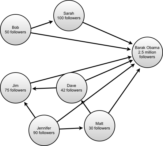
The difference between a weighted graph and a sparse matrix is mostly one of visualization rather than of data. We conceptualize a matrix to be something different than a graph — a matrix is a huge field of rows and columns and a graph a sprawling series of interconnections, but in fact, a sparse matrix and a weighted graph are almost the same thing and easily convertible when viewed from a data-perspective.
So, if we’re thinking of a user’s product ratings as a sparse vector that maps to each product, we can easily model that as a series of weighted edges from the user to each product. In fact, it’d be difficult to produce a tighter format for storing a sparse matrix than a list of connections since we’re able to avoid things like pointers to the next used vector dimension and munge the weights into the same integer value that we use to represent a graph edge.
Beyond that, a graph model allows for us to do some more wild clustering than you’d typically get if you’re imagining the ratings set as a matrix. We can look at things that are not just one, but a couple levels out in the connection structure to figure out how things are related. This is one of the mechanisms that we use to mitigate the “cold start” problem that is endemic to typical collaborative filtering algorithms.
Al fine
I’m tired of writing, you’re tired of reading. If you’ve got questions or have The Killer Application in mind for such a beast, feel free to drop us a line via comments or mail or ping us on Twitter.
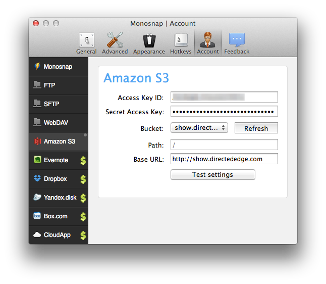
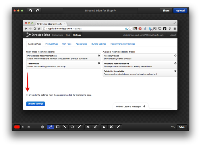 Monosnap itself is pretty straightforward. You take screenshots, potentially annotate them and it uploads them somewhere. Â It hearkens to the Skitch of old. Â However, instead of only uploading images to its own server, it also allows you to upload images to various cloud services.

 Follow us on Twitter
 Fan us on Facebook










 Â
 

